Variational Autoencoders
Variational Auto-Encoders (VAE) [VAEKW13] is one of the most widely used deep generative models. In this tutorial, we show how to implement VAE in ZhuSuan step by step. The full script is at examples/variational_autoencoders/vae.py.
The generative process of a VAE for modeling binarized MNIST data is as follows:
This generative process is a stereotype for deep generative models, which starts with a latent representation (\(z\)) sampled from a simple distribution (such as standard Normal). Then the samples are forwarded through a deep neural network (\(f_{NN}\)) to capture the complex generative process of high dimensional observations such as images. Finally, some noise is added to the output to get a tractable likelihood for the model. For binarized MNIST, the observation noise is chosen to be Bernoulli, with its parameters output by the neural network.
Build the model
In ZhuSuan, a model is constructed using
BayesianNet, which describes a directed
graphical model, i.e., Bayesian networks.
The suggested practice is to wrap model construction into a function (
we shall see the meanings of these arguments soon):
import zhusuan as zs

def build_gen(x_dim, z_dim, n, n_particles=1):
    bn = zs.BayesianNet()
Following the generative process, first we need a standard Normal
distribution to generate the latent representations (\(z\)).
As presented in our graphical model, the data is generated in batches with
batch size n, and for each data, the latent representation is of
dimension z_dim.
So we add a stochastic node by bn.normal to generate samples of shape
[n, z_dim]:
# z ~ N(z|0, I)
z_mean = tf.zeros([n, z_dim])
z = bn.normal("z", z_mean, std=1., group_ndims=1, n_samples=n_particles)
The method bn.normal is a helper function that creates a
Normal distribution and adds a
stochastic node that follows this distribution to the
BayesianNet instance.
The returned z is a StochasticTensor, which
is Tensor-like and can be mixed with Tensors and fed into almost any
Tensorflow primitives.
Note
To learn more about Distribution and
BayesianNet. Please refer to
Basic Concepts in ZhuSuan.
The shape of z_mean is [n, z_dim], which means that
we have [n, z_dim] independent inputs fed into the univariate
Normal distribution.
Because the input parameters are allowed to
broadcast
to match each other’s shape, the standard deviation std is simply set to
1.
Thus the shape of samples and probabilities evaluated at this node should
be of shape [n, z_dim]. However, what we want in modeling MNIST data, is a
batch of [n] independent events, with each one producing samples of z
that is of shape [z_dim], which is the dimension of latent representations.
And the probabilities in every single event in the batch should be evaluated
together, so the shape of local probabilities should be [n] instead of
[n, z_dim].
In ZhuSuan, the way to achieve this is by setting group_ndims`, as we do
in the above model definition code.
To help understand this, several other examples can be found in Distribution
tutorial.
n_samples is the number of samples to generate.
It is None by default, in which case a single sample is generated
without adding a new dimension.
Then we build a neural network of two fully-connected layers with \(z\) as the input, which is supposed to learn the complex transformation that generates images from their latent representations:
# x_logits = f_NN(z)
h = tf.layers.dense(z, 500, activation=tf.nn.relu)
h = tf.layers.dense(h, 500, activation=tf.nn.relu)
x_logits = tf.layers.dense(h, x_dim)
Next, we add an observation distribution (noise) that follows the Bernoulli distribution to get a tractable likelihood when evaluating the probability of an image:
# x ~ Bernoulli(x|sigmoid(x_logits))
bn.bernoulli("x", x_logits, group_ndims=1)
Note
The Bernoulli distribution
accepts log-odds of probabilities instead of probabilities.
This is designed for numeric stability reasons. Similar tricks are used in
Categorical , which accepts
log-probabilities instead of probabilities.
Putting together, the code for constructing a VAE is:
def build_gen(x_dim, z_dim, n, n_particles=1):
    bn = zs.BayesianNet()
    z_mean = tf.zeros([n, z_dim])
    z = bn.normal("z", z_mean, std=1., group_ndims=1, n_samples=n_particles)
    h = tf.layers.dense(z, 500, activation=tf.nn.relu)
    h = tf.layers.dense(h, 500, activation=tf.nn.relu)
    x_logits = tf.layers.dense(h, x_dim)
    bn.bernoulli("x", x_logits, group_ndims=1)
Reuse the model
Unlike common deep learning models (MLP, CNN, etc.), which is for supervised
tasks, a key difficulty in designing programing primitives for generative
models is their inner reusability.
This is because in a probabilistic graphical model, a stochastic node can
have two kinds of states, observed or latent.
Consider the above case, if z is a tensor sampled from the prior, how
about when you meet the condition that z is observed?
In common practice of tensorflow programming, one has to build another
computation graph from scratch and reuse the Variables (weights here).
If there are many stochastic nodes in the model, this process will be really
painful.
We provide a solution for this. To observe any stochastic nodes,
pass a dictionary mapping of (name, Tensor) pairs when constructing
BayesianNet.
This will assign observed values to corresponding StochasticTensor s.
For example, to observe a batch of images x_batch, write:
bn = zs.BayesianNet(observed={"x": x_batch})
Note
The observation passed must have the same type and shape as the StochasticTensor.
However, we usually need to pass different configurations of observations to
the same BayesianNet more than once.
To achieve this, ZhuSuan provides a new class called
MetaBayesianNet
to represent the meta version of BayesianNet
which can repeatedly produce BayesianNet
objects by accepting different observations.
The recommended way to construct a
MetaBayesianNet is by wrapping the
function with a meta_bayesian_net()
decorator:
@zs.meta_bayesian_net(scope="gen")
def build_gen(x_dim, z_dim, n, n_particles=1):
    ...
    return bn

model = build_gen(x_dim, z_dim, n, n_particles)
which transforms the function into returning a
MetaBayesianNet instance:
>>> print(model)
<zhusuan.framework.meta_bn.MetaBayesianNet object at ...
so that we can observe stochastic nodes in this way:
# no observation
bn1 = model.observe()

# observe x
bn2 = model.observe(x=x_batch)
Each time the function is called, a different observation assignment is used
to construct a BayesianNet instance.
One question you may have in mind is that if there are Tensorflow
Variables
created in the above function, will them be reused across these bn s?
The answer is no by default, but you can enable this by switching on the
reuse_variables option in the decorator:
@zs.meta_bayesian_net(scope="gen", reuse_variables=True)
def build_gen(x_dim, z_dim, n, n_particles=1):
    ...
    return bn

model = build_gen(x_dim, z_dim, n, n_particles)
Then bn1 and bn2 will share the same set of Tensorflow Variables.
Note
This only shares Tensorflow Variables across different
BayesianNet instances generated by the same
MetaBayesianNet through the
observe() method.
Creating multiple MetaBayesianNet
objects will recreate the tensorflow Variables, for example, in
m = build_gen(x_dim, z_dim, n, n_particles)
bn = m.observe()

m_new = build_gen(x_dim, z_dim, n, n_particles)
bn_new = m_new.observe()
bn and bn_new will use a different set of Tensorflow
Variables.
Since reusing Tensorflow Variables in repeated function calls is a typical
need, we provide another decorator
reuse_variables() for the more general cases.
Any function decorated by reuse_variables()
will automatically create Tensorflow Variables the first time they are called
and reuse them thereafter.
Inference and learning
Having built the model, the next step is to learn it from binarized MNIST images. We conduct Maximum Likelihood learning, that is, we are going to maximize the log likelihood of data in our model:
where \(\theta\) is the model parameter.
Note
In this variational autoencoder, the model parameter is the network
weights, in other words, it’s the Tensorflow Variables created in the
fully_connected layers.
However, the model we defined has not only the observation (\(x\)) but also latent representation (\(z\)). This makes it hard for us to compute \(p_{\theta}(x)\), which we call the marginal likelihood of \(x\), because we only know the joint likelihood of the model:
while computing the marginal likelihood requires an integral over latent representation, which is generally intractable:
The intractable integral problem is a fundamental challenge in learning latent variable models like VAEs. Fortunately, the machine learning society has developed many approximate methods to address it. One of them is Variational Inference. As the intuition is very simple, we briefly introduce it below.
Because directly optimizing \(\log p_{\theta}(x)\) is infeasible, we choose to optimize a lower bound of it. The lower bound is constructed as
where \(q_{\phi}(z|x)\) is a user-specified distribution of \(z\) (called variational posterior) that is chosen to match the true posterior \(p_{\theta}(z|x)\). The lower bound is equal to the marginal log likelihood if and only if \(q_{\phi}(z|x) = p_{\theta}(z|x)\), when the Kullback–Leibler divergence between them (\(\mathrm{KL}(q_{\phi}(z|x)\|p_{\theta}(z|x))\)) is zero.
Note
In Bayesian Statistics, the process represented by the Bayes’ rule
is called Bayesian Inference, where \(p(z)\) is called the prior, \(p(x|z)\) is the conditional likelihood, \(p(x)\) is the marginal likelihood or evidence, and \(p(z|x)\) is known as the posterior.
This lower bound is usually called Evidence Lower Bound (ELBO). Note that the only probabilities we need to evaluate in it is the joint likelihood and the probability of the variational posterior.
In variational autoencoder, the variational posterior (\(q_{\phi}(z|x)\)) is also parameterized by a neural network (\(g\)), which accepts input \(x\), and outputs the mean and variance of a Normal distribution:
In ZhuSuan, the variational posterior can also be defined as a
BayesianNet . The code for above definition is:
@zs.reuse_variables(scope="q_net")
def build_q_net(x, z_dim, n_z_per_x):
    bn = zs.BayesianNet()
    h = tf.layers.dense(tf.cast(x, tf.float32), 500, activation=tf.nn.relu)
    h = tf.layers.dense(h, 500, activation=tf.nn.relu)
    z_mean = tf.layers.dense(h, z_dim)
    z_logstd = tf.layers.dense(h, z_dim)
    bn.normal("z", z_mean, logstd=z_logstd, group_ndims=1, n_samples=n_z_per_x)
    return bn

variational = build_q_net(x, z_dim, n_particles)
Having both model and variational, we can build the lower bound as:
lower_bound = zs.variational.elbo(
    model, {"x": x}, variational=variational, axis=0)
The returned lower_bound is an
EvidenceLowerBoundObjective
instance, which is also Tensor-like and can be evaluated directly. However,
optimizing this lower bound objective needs special care.
The easiest way is to do
stochastic gradient descent
(SGD), which is very common in deep learning literature.
However, the gradient computation here involves taking derivatives of an
expectation, which needs Monte Carlo estimation.
This often induces large variance if not properly handled.
Note
Directly using auto-differentiation to compute the gradients of
EvidenceLowerBoundObjective
often gives you the wrong results.
This is because auto-differentiation is not designed to handle
expectations.
Many solutions have been proposed to estimate the gradient of some
type of variational lower bound (ELBO or others) with relatively low variance.
To make this more automatic and easier to handle, ZhuSuan has wrapped these
gradient estimators all into methods of the corresponding
variational objective (e.g., the
EvidenceLowerBoundObjective).
These functions don’t return gradient estimates but a more convenient
surrogate cost.
Applying SGD on this surrogate cost with
respect to parameters is equivalent to optimizing the
corresponding variational lower bounds using the well-developed low-variance
estimator.
Here we are using the Stochastic Gradient Variational Bayes (SGVB)
estimator from the original paper of variational autoencoders
[VAEKW13].
This estimator takes benefits of a clever reparameterization trick to
greatly reduce the variance when estimating the gradients of ELBO.
In ZhuSuan, one can use this estimator by calling the method
sgvb()
of the class:~zhusuan.variational.exclusive_kl.EvidenceLowerBoundObjective
instance.
The code for this part is:
# the surrogate cost for optimization
cost = tf.reduce_mean(lower_bound.sgvb())

# the lower bound value to print for monitoring convergence
lower_bound = tf.reduce_mean(lower_bound)
Note
For readers who are interested, we provide a detailed explanation of the
sgvb()
estimator used here, though this is not required for you to use
ZhuSuan’s variational functionality.
The key of SGVB estimator is a reparameterization trick, i.e., they reparameterize the random variable \(z\sim q_{\phi}(z|x) = \mathrm{N}(z|\mu_z(x;\phi), \sigma^2_z(x;\phi))\), as
In this way, the expectation can be rewritten with respect to \(\epsilon\):
Thus the gradients with variational parameters \(\phi\) can be directly moved into the expectation, enabling an unbiased low-variance Monte Carlo estimator:
where \(\epsilon_i \sim \mathrm{N}(0, I)\)
Now that we have had the cost, the next step is to do the stochastic gradient descent. Tensorflow provides many advanced optimizers that improves the plain SGD, among which Adam [VAEKB14] is probably the most popular one in deep learning society. Here we are going to use Tensorflow’s Adam optimizer to do the learning:
optimizer = tf.train.AdamOptimizer(0.001)
infer_op = optimizer.minimize(cost)
Generate images
What we’ve done above is to define and learn the model. To see how it
performs, we would like to let it generate some images in the learning process.
To improve the visual quality of generation, we remove the observation noise,
i.e., the Bernoulli distribution.
We do this by using the direct output of the neural network (x_logits):
@zs.meta_bayesian_net(scope="gen", reuse_variables=True)
def build_gen(x_dim, z_dim, n, n_particles=1):
    bn = zs.BayesianNet()
        ...
    x_logits = tf.layers.dense(h, x_dim)
        ...
and adding a sigmoid function to it to get a “mean” image.
After that, we add a deterministic node in bn to keep track of
the Tensor x_mean:
@zs.meta_bayesian_net(scope="gen", reuse_variables=True)
def build_gen(x_dim, z_dim, n, n_particles=1):
    bn = zs.BayesianNet()
        ...
    x_logits = tf.layers.dense(h, x_dim)
    bn.deterministic("x_mean", tf.sigmoid(x_logits))
        ...
so that we can easily access it from a
BayesianNet instance.
For random generations, no observation about the model is made, so we
construct the corresponding BayesianNet by:
bn_gen = model.observe()
Then the generated samples can be fetched from the x_mean node of
bn_gen:
x_gen = tf.reshape(bn_gen["x_mean"], [-1, 28, 28, 1])
Run gradient descent
Now, everything is good before a run. So we could just open the Tensorflow session, run the training loop, print statistics, and write generated images to disk:
with tf.Session() as sess:
    sess.run(tf.global_variables_initializer())

    for epoch in range(1, epochs + 1):
        time_epoch = -time.time()
        np.random.shuffle(x_train)
        lbs = []
        for t in range(iters):
            x_batch = x_train[t * batch_size:(t + 1) * batch_size]
            _, lb = sess.run([infer_op, lower_bound],
                             feed_dict={x_input: x_batch,
                                        n_particles: 1,
                                        n: batch_size})
            lbs.append(lb)
        time_epoch += time.time()
        print("Epoch {} ({:.1f}s): Lower bound = {}".format(
            epoch, time_epoch, np.mean(lbs)))


        if epoch % save_freq == 0:
            images = sess.run(x_gen, feed_dict={n: 100, n_particles: 1})
            name = os.path.join(result_path,
                                "vae.epoch.{}.png".format(epoch))
            save_image_collections(images, name)
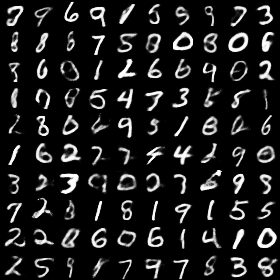
Below is a sample image of random generations from the model. Keep watching them and have fun :)
References
| [VAEKW13] | (1, 2) Diederik P Kingma and Max Welling. Auto-encoding variational bayes. arXiv preprint arXiv:1312.6114, 2013. |
| [VAEKB14] | Diederik Kingma and Jimmy Ba. Adam: a method for stochastic optimization. arXiv preprint arXiv:1412.6980, 2014. |