Logistic Normal Topic Models
The full script for this tutorial is at examples/topic_models/lntm_mcem.py.
An introduction to topic models and Latent Dirichlet Allocation
Nowadays it is much easier to get large corpus of documents. Even if there are no suitable labels with these documents, much information can be extracted. We consider designing a probabilistic model to generate the documents. Generative models can bring more benefits than generating more data. One can also fit the data under some specific structure through generative models. By inferring the parameters in the model (either return a most probable value or figure out its distribution), some valuable information may be discovered.
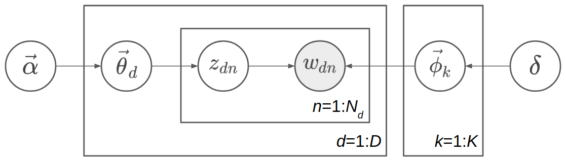
For example, we can model documents as arising from multiple topics, where a topic is defined to be a distribution over a fixed vocabulary of terms. The most famous model is Latent Dirichlet Allocation (LDA) [LNTMBNJ03]. First we describe the notations. Following notations differ from the standard notations in two places for consistence with our notations of LNTM: The topics is denoted \(\vec{\phi}\) instead of \(\vec{\beta}\), and the scalar Dirichlet prior of topics is \(\delta\) instead of \(\eta\). Suppose there are \(D\) documents in the corpus, and the \(d\)th document has \(N_d\) words. Let \(K\) be a specified number of topics, \(V\) the size of vocabulary, \(\vec{\alpha}\) a positive \(K\) dimension-vector, and \(\delta\) a positive scalar. Let \(\mathrm{Dir}_K(\vec{\alpha})\) denote a \(K\)-dimensional Dirichlet with vector parameter \(\vec{\alpha}\) and \(\mathrm{Dir}_V(\delta)\) denote a \(V\)-dimensional Dirichlet with scalar parameter \(\delta\). Let \(\mathrm{Catg}(\vec{p})\) be a categorical distribution with vector parameter \(\vec{p}=(p_1,p_2,...,p_n)^T\) (\(\sum_{i=1}^n p_i=1\)) and support \(\{1,2,...,n\}\).
Note
Sometimes, the categorical and multinomial distributions are conflated, and it is common to speak of a “multinomial distribution” when a “categorical distribution” would be more precise. These two distributions are distinguished in ZhuSuan.
The generative process is:
In more detail, we first sample \(K\) topics \(\{\vec{\phi}_k\}_{k=1}^K\) from the symmetric Dirichlet prior with parameter \(\delta\), so each topic is a \(K\)-dimensional vector, whose components sum up to 1. These topics are shared among different documents. Then for each document, suppose it is the \(d\)th document, we sample a topic proportion vector \(\vec{\theta}_d\) from the Dirichlet prior with parameter \(\vec{\alpha}\), indicating the topic proportion of this document, such as 70% topic 1 and 30% topic 2. Next we start to sample the words in the document. Sampling each word \(w_{dn}\) is a two-step process: first, sample the topic assignment \(z_{dn}\) from the categorical distribution with parameter \(\vec{\theta}_d\); secondly, sample the word \(w_{dn}\) from the categorical distribution with parameter \(\vec{\phi}_{z_{dn}}\). The range of \(d\) is \(1\) to \(D\), and the range of \(n\) is \(1\) to \(N_d\) in the \(d\)th document. The model is shown as a directed graphical model in the following figure.
Note
Topic \(\{\phi_k\}\), topic proportion \(\{\theta_d\}\), and topic assignment \(\{z_{dn}\}\) have very different meaning. Topic means some distribution over the words in vocabulary. For example,a topic consisting of 10% “game”, 5% “hockey”, 3% “team”, …, possibly means a topic about sports. They are shared among different documents. A topic proportion belongs to a document, roughly indicating the probability distribution of topics in the document. A topic assignment belongs to a word in a document, indicating when sampling the word, which topic is sampled first, so the word is sampled from this assigned topic. Both topic, topic proportion, and topic assignment are latent variables which we have not observed. The only observed variable in the generative model is the words \(\{w_{dn}\}\), and what Bayesian inference needs to do is to infer the posterior distribution of topic \(\{\phi_k\}\), topic proportion \(\{\theta_d\}\), and topic assignment \(\{z_{dn}\}\).
The key property of LDA is conjugacy between the Dirichlet prior and likelihood. We can write the joint probability distribution as follows:
Here \(p(y|x)\) means conditional distribution in which \(x\) is a random variable, but \(p(y;x)\) means distribution parameterized by \(x\), while \(x\) is a fixed value.
We denote \(\mathbf{\Theta}=(\vec{\theta}_1, \vec{\theta}_2, ..., \vec{\theta}_D)^T\), \(\mathbf{\Phi}=(\vec{\phi}_1, \vec{\phi}_2, ..., \vec{\phi}_K)^T\). Then \(\mathbf{\Theta}\) is a \(D\times K\) matrix with each row representing topic proportion of one document, while \(\mathbf{\Phi}\) is a \(K\times V\) matrix with each row representing a topic. We also denote \(\mathbf{z}=z_{1:D,1:N}\) and \(\mathbf{w}=w_{1:D,1:N}\) for convenience.
Our goal is to do posterior inference from the joint distribution. Since there are three sets of latent variables in the joint distribution: \(\mathbf{\Theta}\), \(\mathbf{\Phi}\) and \(\mathbf{z}\), inferring their posterior distribution at the same time will be difficult, but we can leverage the conjugacy between Dirichlet prior such as \(p(\vec{\theta}_d; \vec{\alpha})\) and the multinomial likelihood such as \(\prod_{n=1}^{N_d} p(z_{dn}|\vec{\theta}_d)\) (here the multinomial refers to a product of a bunch of categorical distribution, i.e. ignore the normalizing factor of multinomial distribution).
Two ways to leverage this conjugacy are:
(1) Iterate by fixing two sets of latent variables, and do conditional computing for the remaining set. The examples are Gibbs sampling and mean-field variational inference. For Gibbs sampling, each iterating step is fixing the value of samples of two sets, and sample from the conditional distribution of the remaining set. For mean-field variational inference, we often optimize by coordinate ascent: each iterating step is fixing the variational distribution of two sets, and updating the variational distribution of the remaining set based on the parameters of the variational distribution of the two sets. Thanks to the conjugacy, both conditional distribution in Gibbs sampling and conditional update of the variational distribution in variational inference are tractable.
(2) Alternatively, we can integrate out some sets of latent variable before doing further inference. For example, we can integrate out \(\mathbf{\Theta}\) and \(\mathbf{\Phi}\), remaining the joint distribution \(p(\mathbf{w}, \mathbf{z}; \vec{\alpha}, \delta)\) and do Gibbs sampling or variational Bayes on \(\mathbf{z}\). After having a estimation to \(\mathbf{z}\), we can extract some estimation about \(\mathbf{\Phi}\) as the topic information too. These methods are called respectively collapsed Gibbs sampling, and collapsed variational Bayesian inference.
However, conjugacy requires the model being designed carefully. Here, we use a more direct and general method to do Bayesian inference: Monte-Carlo EM, with HMC [LNTMN+11] as the Monte-Carlo sampler.
Logistic Normal Topic Model in ZhuSuan
Integrating out \(\mathbf{\Theta}\) and \(\mathbf{\Phi}\) requires conjugacy, or the integration is intractable. But integrating \(\mathbf{z}\) is always tractable since \(\mathbf{z}\) is discrete. Now we have:
More compactly,
which means when sampling the words in the \(d\)th document, the word distribution is the weighted average of all topics, and the weights are the topic proportion of the document.
In LDA we implicitly use the bag-of-words model, and here we make it explicit. Let \(\vec{x}_d\) be a \(V\)-dimensional vector, \(\vec{x}_d=\sum_{n=1}^{N_d}\mathrm{one\_hot}(w_{dn})\). That is, for \(v\) from \(1\) to \(V\), \((\vec{x}_d)_v\) represents the occurence count of the \(v\)th word in the document. Denote \(\mathbf{X}=(\vec{x}_1, \vec{x}_2, ..., \vec{x}_D)^T\), which is a \(D\times V\) matrix. You can verify the following concise formula:
Here, CE means cross entropy, which is defined for matrices as \(\mathrm{CE}(\mathbf{A},\mathbf{B})=-\sum_{i,j}A_{ij}\log B_{ij}\). Note that \(p(\mathbf{X}|\mathbf{\Theta}, \mathbf{\Phi})\) is not a proper distribution; It is a convenient term representing the likelihood of parameters. What we actually means is \(\log p(w_{1:D,1:N}|\mathbf{\Theta}, \mathbf{\Phi})=-\mathrm{CE}(\mathbf{X}, \mathbf{\Theta}\mathbf{\Phi})\).
A intuitive demonstration of \(\mathbf{\Theta}\), \(\mathbf{\Phi}\) and \(\mathbf{\Theta\Phi}\) is shown in the following picture. \(\mathbf{\Theta}\) is the document-topic matrix, \(\mathbf{\Phi}\) is the topic-word matrix, and then \(\mathbf{\Theta\Phi}\) is the document-word matrix, which contains the word sampling distribution of each document.

As minimizing the cross entropy encourages \(\mathbf{X}\) and \(\mathbf{\Theta}\mathbf{\Phi}\) to be similar, this may remind you of low-rank matrix factorization. It is natural since topic models can be interpreted as learning “document-topics” parameters and “topic-words” parameters. In fact one of the earliest topic models are solved using SVD, a standard algorithm for low-rank matrix factorization. However, as a probabilistic model, our model is different from matrix factorization by SVD (e.g. the loss function is different). Probabilistic model is more interpretable and can be solved by more algorithms, and Bayesian model can bring the benefits of incorporating prior knowledge and inferring with uncertainty.
After integrating \(\mathbf{z}\), only \(\mathbf{\Theta}\) and \(\mathbf{\Phi}\) are left, and there is no conjugacy any more. Even if we apply the “conditional computing” trick like Gibbs sampling, no closed-form updating process can be obtained. However, we can adopt the gradient-based method such as HMC and gradient ascent. Note that each row of \(\mathbf{\Theta}\) and \(\mathbf{\Phi}\) lies on a probability simplex, which is bounded and embedded. It is not common for HMC or gradient ascent to deal with constrained sampling or constrained optimzation. Since we do not nead conjugacy now, we replace the Dirichlet prior with logistic normal prior. Now the latent variables live in the whole space \(\mathbb{R}^n\).
One may ask why to integrate the parameters \(\mathbf{z}\) and lose the conjugacy. That is because our inference technique can also apply to other models which do not have conjugacy from the beginning, such as Neural Variational Document Model ([LNTMMYB16]).
The logistic normal topic model can be described as follows, where \(\vec{\beta}_k\) is \(V\)-dimensional and \(\vec{\eta}_d\) is \(K\)-dimensional:
The graphical model representation is shown in the following figure.
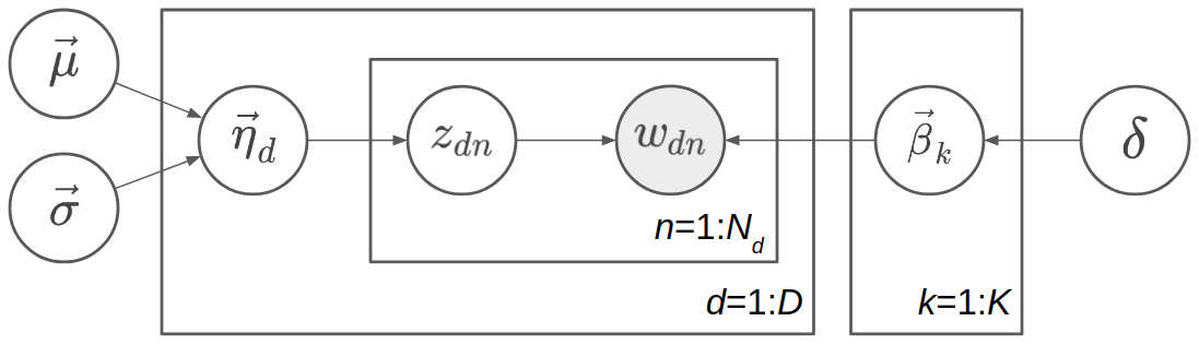
Since \(\vec{\theta}_d\) is a deterministic function of \(\vec{\eta}_d\), we can omit one of them in the probabilistic graphical model representation. Here \(\vec{\theta}_d\) is omitted because \(\vec{\eta}_d\) has a simpler prior. Similarly, we omit \(\vec{\phi}_k\) and keep \(\vec{\beta}_k\).
Note
Called Logistic Normal Topic Model, maybe this reminds you of correlated topic models. However, in our model the normal prior of \(\vec{\eta}_d\) has a diagonal covariance matrix \(\mathrm{diag}(\vec{\sigma}^2)\), so it cannot model the correlations between different topics in the corpus. However, logistic normal distribution can approximate Dirichlet distribution (see [LNTMSS17]). Hence our model is roughly the same as LDA, while the inference techniques are different.
We denote \(\mathbf{H}=(\vec{\eta}_1, \vec{\eta}_2, ..., \vec{\eta}_D)^T\), \(\mathbf{B}=(\vec{\beta}_1, \vec{\beta}_2, ..., \vec{\beta}_K)^T\). Then \(\mathbf{\Theta}=\mathrm{softmax}(\mathbf{H})\), and \(\mathbf{\Phi}=\mathrm{softmax}(\mathbf{B})\). Recall our notation that \(\mathbf{X}=(\vec{x}_1, \vec{x}_2, ..., \vec{x}_D)^T\) where \(\vec{x}_d=\sum_{n=1}^{N_d}\mathrm{one\_hot}(w_{dn})\). After integrating \(\{z_{dn}\}\), the last two lines of the generating process:
become \(\log p(\mathbf{X}|\mathbf{\Theta}, \mathbf{\Phi})=-\mathrm{CE}(\mathbf{X}, \mathbf{\Theta}\mathbf{\Phi})\). So we can write the joint probability distribution as follows:
where both \(p(\mathbf{B}; \delta)\) and \(p(\mathbf{H}; \vec{\mu}, \vec{\sigma})\) are Gaussian distribution and \(p(\mathbf{X}|\mathbf{H}, \mathbf{B})=-\mathrm{CE}(\mathbf{X}, \mathrm{softmax}(\mathbf{H})\mathrm{softmax}(\mathbf{B}))\).
In ZhuSuan, the code for constructing such a model is:
@zs.meta_bayesian_net(scope='lntm')
def lntm(n_chains, n_docs, n_topics, n_vocab, eta_mean, eta_logstd):
    bn = zs.BayesianNet()
    eta_mean = tf.tile(tf.expand_dims(eta_mean, 0), [n_docs, 1])
    eta = bn.normal('eta', eta_mean, logstd=eta_logstd, n_samples=n_chains,
                    group_ndims=1)
    theta = tf.nn.softmax(eta)
    beta = bn.normal('beta', tf.zeros([n_topics, n_vocab]),
                    logstd=log_delta, group_ndims=1)
    phi = tf.nn.softmax(beta)
    # doc_word: Document-word matrix
    doc_word = tf.matmul(tf.reshape(theta, [-1, n_topics]), phi)
    doc_word = tf.reshape(doc_word, [n_chains, n_docs, n_vocab])
    bn.unnormalized_multinomial('x', tf.log(doc_word), normalize_logits=False,
                                dtype=tf.float32)
    return bn
where eta_mean is \(\vec{\mu}\), eta_logstd is \(\log\vec{\sigma}\),
eta is \(\mathbf{H}\) (\(\mathrm{H}\) is the uppercase letter of
\(\mathrm{\eta}\)), theta is
\(\mathbf{\Theta}=\mathrm{softmax}(\mathbf{H})\), beta is \(\mathbf{B}\)
(\(\mathrm{B}\) is the uppercase letter of \(\mathrm{\beta}\)), phi
is \(\mathbf{\Phi}=\mathrm{softmax}(\mathbf{B})\), doc_word is
\(\mathbf{\Theta}\mathbf{\Phi}\), x is \(\mathbf{X}\).
Q: What does UnnormalizedMultinomial distribution means?
A: UnnormalizedMultinomial distribution is not a proper distribution. It
means the likelihood of “bags of categorical”. To understand this, let’s
talk about multinomial distribution first. Suppose there are \(k\) events
\(\{1,2,...,k\}\) with the probabilities \(p_1,p_2,...,p_k\), and we do
\(n\) trials, and the count of result being \(i\) is \(x_i\). Denote
\(\vec{x}=(x_1,x_2,...,x_k)^T\) and \(\vec{p}=(p_1,p_2,...,p_k)^T\).
Then \(\vec{x}\) follows multinomial distribution: \(p(\vec{x};
\vec{p})=\frac{n!}{x_1!...x_k!}p_1^{x_1}...p_k^{x_k}\), so \(\log p(\vec{x};
\vec{p})=\log\frac{n!}{x_1!...x_k!} - \mathrm{CE}(\vec{x},\vec{p})\). However,
when we want to optimize the parameter \(\vec{p}\), we do not care the first
term. On the other hand, if we have a sequence of results \(\vec{w}\), and
the result counts are summarized in \(\vec{x}\). Then \(\log p(\vec{w};
\vec{p})=-\mathrm{CE}(\vec{x},\vec{p})\). The normalizing constant also
disappears. Since sometimes we only have access to \(\vec{x}\) instead of
the actual sequence of results, when we want to optimize w.r.t. the parameters,
we can write \(\vec{x}\sim \mathrm{UnnormalizedMultinomial}(\vec{p})\),
although it is not a proper distribution and we cannot sample from it.
UnnormalizedMultinomial just means \(p(\vec{w};
\vec{p})=-\mathrm{CE}(\vec{x},\vec{p})\). In the example of topic models, the
situation is also like this.
Q: The shape of eta in the model is n_chains*n_docs*n_topics. Why we
need the first dimension to store its different samples?
A: After introducing the inference method, we should know eta is a latent
variable which we need to integrate w.r.t. its distribution. In many cases the
integration is intractable, so we replace the integration with Monte-Carlo
methods, which requires the samples of the latent variable. Therefore we need to
construct our model, calculate the joint likelihood and do inference all with
the extra dimension storing different samples. In this example, the extra
dimension is called “chains” because we utilize the extra dimension to initialize
multiple chains and perform HMC evolution on each chain, in order to do parallel
sampling and to get independent samples from the posterior.
Inference
Let’s analyze the parameters and latent variables in the joint distribution. \(\delta\) controls the sparsity of the words included in each topic, and larger \(\delta\) leads to more sparsity. We leave it as a given tunable hyperparameter without the need to optimize. The parameters we need to optimize is \(\vec{\mu}\) and \(\vec{\sigma}^2\), whose element represents the mean and variance of topic proportion in documents; and \(\mathbf{B}\), which represents the topics. For \(\vec{\mu}\) and \(\vec{\sigma}\), we want to find their maximum likelihood (MLE) solution. Unlike \(\vec{\mu}\) and \(\vec{\sigma}\), \(\mathbf{B}\) has a prior, so we could treat it as a random variable and infer its posterior distribution. But here we just find its maximum a posterior (MAP) estimation, so we treat it as a parameter and optimize it by gradient ascent instead of inference via HMC. \(\mathbf{H}\) is the latent variable, so we want to integrate it out before doing optimization.
Therefore, after integrating \(\mathbf{H}\), our optimization problem is:
where
The term \(\log p(\mathbf{X}| \mathbf{B}; \vec{\mu}, \vec{\sigma}) = \log \int_{\mathbf{H}} p(\mathbf{X}, \mathbf{H}| \mathbf{B}; \vec{\mu}, \vec{\sigma}) d\mathbf{H}\) is evidence of the observed data \(\mathbf{X}\), given the model with parameters \(\mathbf{B}\), \(\vec{\mu}\), \(\vec{\sigma}\). Computing the integration is intractable, let alone maximize it w.r.t. the parameters. Fortunately, this is the standard form of which we can write an lower bound called evidence lower bound (ELBO):
Therefore,
When \(q(\mathbf{H})=p(\mathbf{H}|\mathbf{X},\mathbf{B}; \vec{\mu}, \vec{\sigma})\), the lower bound is tight. To do optimization, we can apply coordinate ascent to the lower bound, i.e. expectation-maximization (EM) algorithm: We iterate between E-step and M-step.
In E-step, let
In M-step, let
However, both the posterior \(p(\mathbf{H}|\mathbf{X},\mathbf{B}; \vec{\mu}, \vec{\sigma})\) in the E step and the integration \(\mathbb{E}_{q(\mathbf{H})}[\log p(\mathbf{X}, \mathbf{H}| \mathbf{B}; \vec{\mu}, \vec{\sigma})]\) in the M step are intractable. It seems that we have turned an intractable problem into another intractable problem.
We have solutions indeed. Since the difficulty lies in calculating and using the posterior, we can use the whole set of tools in Bayesian inference. Here we use sampling methods, to draw a series of samples \(\mathbf{H}^{(1)}, \mathbf{H}^{(2)}, ..., \mathbf{H}^{(S)}\) from \(p(\mathbf{H}|\mathbf{X},\mathbf{B}; \vec{\mu}, \vec{\sigma})\). Then we let \(q(\mathbf{H})\) be the empirical distribution of these samples, as an approximation to the true posterior. Then the M-step becomes:
Now the objective function is tractable to compute. This variant of EM algorithm is called Monte-Carlo EM.
We analyze the E-step and M-step in more detail. What sampling method should we choose in E-step? One of the workhorse sampling methods is Hamiltonian Monte Carlo (HMC) [LNTMN+11]. Unlike Gibbs sampling which needs a sampler of the conditional distribution, HMC is a black-box method which only requires access to the gradient of log joint distribution at any position, which is almost always tractable as long as the model is differentiable and the latent variable is unconstrained.
To use HMC in ZhuSuan, first define the HMC object with its parameters:
hmc = zs.HMC(step_size=1e-3, n_leapfrogs=20, adapt_step_size=True,
             target_acceptance_rate=0.6)
Then write the log joint probability \(\log p(\mathbf{X},\mathbf{H}| \mathbf{B}; \vec{\mu}, \vec{\sigma})= \log p(\mathbf{X}| \mathbf{B},\mathbf{H}) + p(\mathbf{H};\vec{\mu}, \vec{\sigma})\):
def e_obj(bn):
    return bn.cond_log_prob('eta') + bn.cond_log_prob('x')
Given the following defined tensor,
x = tf.placeholder(tf.float32, shape=[batch_size, n_vocab], name='x')
eta = tf.Variable(tf.zeros([n_chains, batch_size, n_topics]), name='eta')
beta = tf.Variable(tf.zeros([n_topics, n_vocab]), name='beta')
we can define the sampling operator of HMC:
model = lntm(n_chains, batch_size, n_topics, n_vocab, eta_mean, eta_logstd)
model.log_joint = e_obj
sample_op, hmc_info = hmc.sample(model,
                                 observed={'x': x, 'beta': beta},
                                 latent={'eta': eta})
When running the session, we can run sample_op to update the value of
eta. Note that the first parameter of hmc.sample is a
MetaBayesianNet instance corresponding to
the generative model. It could also be a function accepting a Python dictionary
containing values of both the observed and latent variables as its argument,
and returning the log joint probability. hmc_info is a struct containing
information about the sampling iteration executed by sample_op, such as the
acceptance rate.
In the M-step, since \(\log p(\mathbf{X},\mathbf{H}| \mathbf{B}; \vec{\mu}, \vec{\sigma})= \log p(\mathbf{X}| \mathbf{B},\mathbf{H}) + p(\mathbf{H};\vec{\mu}, \vec{\sigma})\), we can write the updating formula in more detail:
Then \(\vec{\mu}\) and \(\vec{\sigma}\) have closed solution by taking the samples of \(\mathbf{H}\) as observed data and do maximum likelihood estimation of parameters in Gaussian distribution. \(\mathbf{B}\), however, does not have a closed-form solution, so we do optimization using gradient ascent.
The gradient ascent operator of \(\mathbf{B}\) can be defined as follows:
bn = model.observe(eta=eta, x=x, beta=beta)
log_p_beta, log_px = bn.cond_log_prob(['beta', 'x'])
log_p_beta = tf.reduce_sum(log_p_beta)
log_px = tf.reduce_sum(tf.reduce_mean(log_px, axis=0))
log_joint_beta = log_p_beta + log_px
learning_rate_ph = tf.placeholder(tf.float32, shape=[], name='lr')
optimizer = tf.train.AdamOptimizer(learning_rate_ph)
infer = optimizer.minimize(-log_joint_beta, var_list=[beta])
Since when optimizing \(\mathbf{B}\), the samples of \(\mathbf{H}\) is
fixed, var_list=[beta] in the last line is necessary.
In the E-step, \(p(\mathbf{H}|\mathbf{X},\mathbf{B}; \vec{\mu}, \vec{\sigma})\) could factorise as \(\prod_{d=1}^D p(\vec{\eta}_d|\vec{x}_d,\mathbf{B}; \vec{\mu}, \vec{\sigma})\), so we can do sampling for a mini-batch of data given some value of global parameters \(\mathbf{B}\), \(\vec{\mu}\), and \(\vec{\sigma}\). Since the update of \(\mathbf{B}\) requires calculating gradients and has a relatively large time cost, we use stochastic gradient ascent to optimize it. That is, after a mini-batch of latent variables are sampled, we do a step of gradient ascent as M-step for \(\mathbf{B}\) using the mini-batch chosen in the E-step.
Now we have both the sampling operator for the latent variable eta and
optimizing operator for the parameter beta, while the optimization w.r.t.
eta_mean and eta_logstd is straightforward. Now we can run the EM
algorithm.
First, the definition is as follows:
iters = X_train.shape[0] // batch_size
Eta = np.zeros((n_chains, X_train.shape[0], n_topics), dtype=np.float32)
Eta_mean = np.zeros(n_topics, dtype=np.float32)
Eta_logstd = np.zeros(n_topics, dtype=np.float32)

eta_mean = tf.placeholder(tf.float32, shape=[n_topics], name='eta_mean')
eta_logstd = tf.placeholder(tf.float32, shape=[n_topics],
                            name='eta_logstd')
eta_ph = tf.placeholder(tf.float32, shape=[n_chains, batch_size, n_topics],
                        name='eta_ph')
init_eta_ph = tf.assign(eta, eta_ph)
The key code in an epoch is:
time_epoch = -time.time()
lls = []
accs = []
for t in range(iters):
    x_batch = X_train[t*batch_size: (t+1)*batch_size]
    old_eta = Eta[:, t*batch_size: (t+1)*batch_size, :]

    # E step
    sess.run(init_eta_ph, feed_dict={eta_ph: old_eta})
    for j in range(num_e_steps):
        _, new_eta, acc = sess.run(
            [sample_op, hmc_info.samples['eta'],
             hmc_info.acceptance_rate],
            feed_dict={x: x_batch,
                       eta_mean: Eta_mean,
                       eta_logstd: Eta_logstd})
        accs.append(acc)
        # Store eta for the persistent chain
        if j + 1 == num_e_steps:
            Eta[:, t*batch_size: (t+1)*batch_size, :] = new_eta

    # M step
    _, ll = sess.run(
        [infer, log_px],
        feed_dict={x: x_batch,
                   eta_mean: Eta_mean,
                   eta_logstd: Eta_logstd,
                   learning_rate_ph: learning_rate})
    lls.append(ll)

# Update hyper-parameters
Eta_mean = np.mean(Eta, axis=(0, 1))
Eta_logstd = np.log(np.std(Eta, axis=(0, 1)) + 1e-6)

time_epoch += time.time()
print('Epoch {} ({:.1f}s): Perplexity = {:.2f}, acc = {:.3f}, '
      'eta mean = {:.2f}, logstd = {:.2f}'
      .format(epoch, time_epoch,
              np.exp(-np.sum(lls) / np.sum(X_train)),
              np.mean(accs), np.mean(Eta_mean),
              np.mean(Eta_logstd)))
We run num_e_steps times of E-step before M-step to make samples of HMC
closer to the desired equilibrium distribution. We print the mean
acceptance rate of HMC to diagnose whether HMC is working properly.
If it is too close to 0 or 1, the quality of samples will often be poor.
Moreover, when HMC works properly, we can also tune the acceptance rate to
a value for better performance, and the value is usually between 0.6 and 0.9.
In the example we set adapt_step_size=True and
target_acceptance_rate=0.6 to HMC, so the outputs of actual acceptance rates
should be close to 0.6.
Finally we can output the optimized value of phi = softmax(beta),
eta_mean and eta_logstd to show the learned topics and their proportion
in the documents of the corpus:
p = sess.run(phi)
for k in range(n_topics):
    rank = list(zip(list(p[k, :]), range(n_vocab)))
    rank.sort()
    rank.reverse()
    sys.stdout.write('Topic {}, eta mean = {:.2f} stdev = {:.2f}: '
                        .format(k, Eta_mean[k], np.exp(Eta_logstd[k])))
    for i in range(10):
        sys.stdout.write(vocab[rank[i][1]] + ' ')
    sys.stdout.write('\n')
Evaluation
The log_likelihood used to calculate the perplexity may be confusing.
Typically, the “likelihood” should refer to the evidence of the observed data
given some parameter value, i.e. \(p(\mathbf{X}| \mathbf{B}; \vec{\mu},
\vec{\sigma})\), with the latent variable \(\mathbf{H}\) integrated. However,
it is even more difficult to compute the marginal likelihood than to do
posterior inference. In the code, the likelihood is actually
\(p(\mathbf{X}|\mathbf{H}, \mathbf{B})\), which is not the marginal
likelihood; we should integrate it w.r.t. the prior of \(\mathbf{H}\) to get
marginal likelihood. Hence the perplexity output during the training process
will be smaller than the actual value.
After training the model and outputing the topics, the script will run Annealed Importance Sampling (AIS) to estimate the marginal likelihood more accurately. It may take some time, and you could turn on the verbose mode of AIS to see its progress. Then our script will output the estimated perplexity which is relatively reliable. We do not introduce AIS here. Readers who are interested could refer to [LNTMNea01].
| [LNTMBNJ03] | David M Blei, Andrew Y Ng, and Michael I Jordan. Latent dirichlet allocation. Journal of machine Learning research, 3(Jan):993–1022, 2003. |
| [LNTMN+11] | (1, 2) Radford M Neal and others. Mcmc using hamiltonian dynamics. Handbook of Markov Chain Monte Carlo, 2011. |
| [LNTMMYB16] | Yishu Miao, Lei Yu, and Phil Blunsom. Neural variational inference for text processing. In International Conference on Machine Learning, 1727–1736. 2016. |
| [LNTMSS17] | Akash Srivastava and Charles Sutton. Autoencoding variational inference for topic models. arXiv preprint arXiv:1703.01488, 2017. |
| [LNTMNea01] | Radford M Neal. Annealed importance sampling. Statistics and computing, 11(2):125–139, 2001. |