Bayesian Neural Networks
Note
This tutorial assumes that readers have been familiar with ZhuSuan’s basic concepts.
Recent years have seen neural networks’ powerful abilities in fitting complex transformations, with successful applications on speech recognition, image classification, and machine translation, etc. However, typical training of neural networks requires lots of labeled data to control the risk of overfitting. And the problem becomes harder when it comes to real world regression tasks. These tasks often have smaller amount of training data to use, and the high-frequency characteristics of these data often makes neural networks easier to get trapped in overfitting.
A principled approach for solving this problem is Bayesian Neural Networks (BNN). In BNN, prior distributions are put upon the neural network’s weights to consider the modeling uncertainty. By doing Bayesian inference on the weights, one can learn a predictor which both fits to the training data and reasons about the uncertainty of its own prediction on test data. In this tutorial, we show how to implement BNNs in ZhuSuan. The full script for this tutorial is at examples/bayesian_neural_nets/bnn_vi.py.
We use a regression dataset called Boston housing. This has \(N = 506\) data points, with \(D = 13\) dimensions. The generative process of a BNN for modeling multivariate regression is as follows:
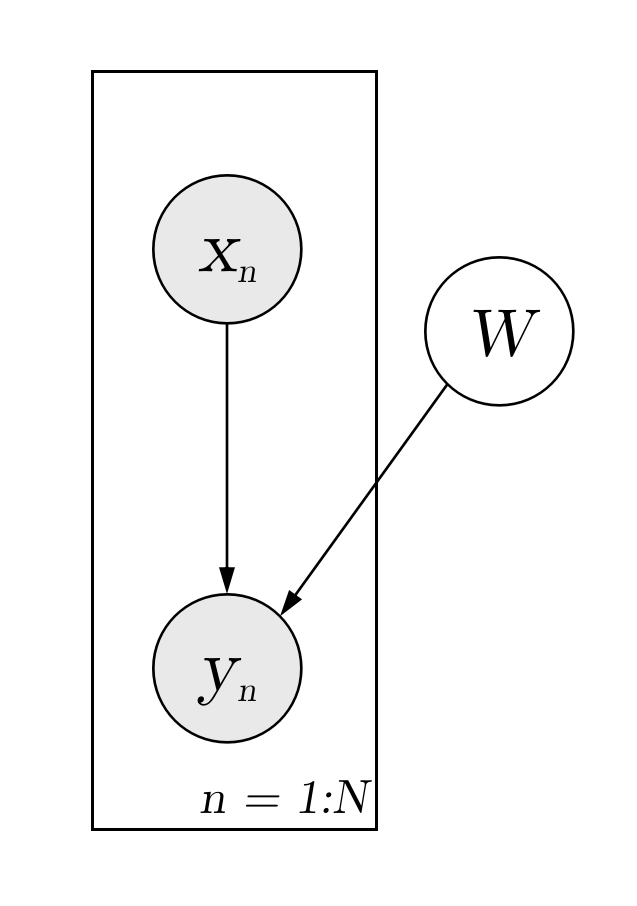
This generative process starts with an input feature (\(x\)), which is forwarded through a deep neural network (\(f_{NN}\)) with \(L\) layers, whose parameters in each layer (\(W_i\)) satisfy a factorized multivariate standard Normal distribution. With this forward transformation, the model is able to learn complex relationships between the input (\(x\)) and the output (\(y\)). Finally, some noise is added to the output to get a tractable likelihood for the model, which is typically a Gaussian noise in regression problems. A graphical model representation for bayesian neural network is as follows.
Build the model
We start by the model building function (we shall see the meanings of these arguments later):
@zs.meta_bayesian_net(scope="bnn", reuse_variables=True)
def build_bnn(x, layer_sizes, n_particles):
    bn = zs.BayesianNet()
Following the generative process, we need standard Normal
distributions to generate the weights (\(\{W_i\}_{i=1}^L\)) in each layer.
For a layer with n_in input units and n_out output units, the weights
are of shape [n_out, n_in + 1] (one additional column for bias).
To support multiple samples (useful in inference and prediction), a common
practice is to set the n_samples argument to a placeholder, which we
choose to be n_particles here:
h = tf.tile(x[None, ...], [n_particles, 1, 1])
for i, (n_in, n_out) in enumerate(zip(layer_sizes[:-1], layer_sizes[1:])):
    w = bn.normal("w" + str(i), tf.zeros([n_out, n_in + 1]), std=1.,
                  group_ndims=2, n_samples=n_particles)
Note that we expand x with a new dimension and tile it to enable
computation with multiple particles of weight samples.
To treat the weights in each layer as a whole and evaluate the probability of
them together, group_ndims is set to 2.
If you are unfamiliar with this property, see Distribution for details.
Then we write the feed-forward process of neural networks, through which the
connection between output y and input x is established:
for i, (n_in, n_out) in enumerate(zip(layer_sizes[:-1], layer_sizes[1:])):
    w = bn.normal("w" + str(i), tf.zeros([n_out, n_in + 1]), std=1.,
                  group_ndims=2, n_samples=n_particles)
    h = tf.concat([h, tf.ones(tf.shape(h)[:-1])[..., None]], -1)
    h = tf.einsum("imk,ijk->ijm", w, h) / tf.sqrt(
        tf.cast(tf.shape(h)[2], tf.float32))
    if i < len(layer_sizes) - 2:
        h = tf.nn.relu(h)
Next, we add an observation distribution (noise) to get a tractable likelihood when evaluating the probability:
y_mean = bn.deterministic("y_mean", tf.squeeze(h, 2))
y_logstd = tf.get_variable("y_logstd", shape=[],
                           initializer=tf.constant_initializer(0.))
bn.normal("y", y_mean, logstd=y_logstd)
Putting together and adding model reuse, the code for constructing a BNN is:
@zs.meta_bayesian_net(scope="bnn", reuse_variables=True)
def build_bnn(x, layer_sizes, n_particles):
    bn = zs.BayesianNet()
    h = tf.tile(x[None, ...], [n_particles, 1, 1])
    for i, (n_in, n_out) in enumerate(zip(layer_sizes[:-1], layer_sizes[1:])):
        w = bn.normal("w" + str(i), tf.zeros([n_out, n_in + 1]), std=1.,
                      group_ndims=2, n_samples=n_particles)
        h = tf.concat([h, tf.ones(tf.shape(h)[:-1])[..., None]], -1)
        h = tf.einsum("imk,ijk->ijm", w, h) / tf.sqrt(
            tf.cast(tf.shape(h)[2], tf.float32))
        if i < len(layer_sizes) - 2:
            h = tf.nn.relu(h)

    y_mean = bn.deterministic("y_mean", tf.squeeze(h, 2))
    y_logstd = tf.get_variable("y_logstd", shape=[],
                               initializer=tf.constant_initializer(0.))
    bn.normal("y", y_mean, logstd=y_logstd)
    return bn
Inference
Having built the model, the next step is to infer the posterior distribution, or uncertainty of weights given the training data.
Because the normalizing constant is intractable, we cannot directly compute the posterior distribution of network parameters (\(\{W_i\}_{i=1}^L\)). In order to solve this problem, we use Variational Inference, i.e., using a variational distribution \(q_{\phi}(\{W_i\}_{i=1}^L)=\prod_{i=1}^L{q_{\phi_i}(W_i)}\) to approximate the true posterior. The simplest variational posterior (\(q_{\phi_i}(W_i)\)) we can specify is factorized (also called mean-field) Normal distribution parameterized by its mean and log standard deviation.
The code for above definition is:
@zs.reuse_variables(scope="variational")
def build_mean_field_variational(layer_sizes, n_particles):
    bn = zs.BayesianNet()
    for i, (n_in, n_out) in enumerate(zip(layer_sizes[:-1], layer_sizes[1:])):
        w_mean = tf.get_variable(
            "w_mean_" + str(i), shape=[n_out, n_in + 1],
            initializer=tf.constant_initializer(0.))
        w_logstd = tf.get_variable(
            "w_logstd_" + str(i), shape=[n_out, n_in + 1],
            initializer=tf.constant_initializer(0.))
        bn.normal("w" + str(i), w_mean, logstd=w_logstd,
                  n_samples=n_particles, group_ndims=2)
    return bn
In Variational Inference, to make \(q_{\phi}(W)\) approximate \(p(W|x_{1:N}, y_{1:N})\) well. We need to maximize a lower bound of the marginal log probability (\(\log p(y|x)\)):
The lower bound is equal to the marginal log likelihood if and only if \(q_{\phi}(W) = p(W|x_{1:N}, y_{1:N})\), for \(i\) in \(1\cdots L\), when the Kullback–Leibler divergence between them (\(\mathrm{KL}(q_{\phi}(W)\|p(W|x_{1:N}, y_{1:N})\)) is zero.
This lower bound is usually called Evidence Lower Bound (ELBO). Note that the only probabilities we need to evaluate in it is the joint likelihood and the probability of the variational posterior. The log conditional likelihood is
Computing log conditional likelihood for the whole dataset is very time-consuming. In practice, we sub-sample a minibatch of data to approximate the conditional likelihood
Here \(\{(x_m, y_m)\}_{m=1:M}\) is a subset including \(M\) random samples from the training set \(\{(x_n, y_n)\}_{n=1:N}\). \(M\) is called the batch size. By setting the batch size relatively small, we can compute the lower bound above efficiently.
Note
Different from models like VAEs, BNN’s latent variables \(\{W_i\}_{i=1}^L\) are global for all the data, therefore we don’t explicitly condition \(W\) on each data in the variational posterior.
We optimize this lower bound by stochastic gradient descent. As we have done in the VAE tutorial, the Stochastic Gradient Variational Bayes (SGVB) estimator is used. The code for this part is:
model = build_bnn(x, layer_sizes, n_particles)
variational = build_mean_field_variational(layer_sizes, n_particles)

def log_joint(bn):
    log_pws = bn.cond_log_prob(w_names)
    log_py_xw = bn.cond_log_prob('y')
    return tf.add_n(log_pws) + tf.reduce_mean(log_py_xw, 1) * n_train

model.log_joint = log_joint

lower_bound = zs.variational.elbo(
    model, {'y': y}, variational=variational, axis=0)
cost = lower_bound.sgvb()

optimizer = tf.train.AdamOptimizer(learning_rate=0.01)
infer_op = optimizer.minimize(cost)
Evaluation
What we’ve done above is to define the model and infer the parameters. The main purpose of doing this is to predict about new data. The probability distribution of new data (\(y\)) given its input feature (\(x\)) and our training data (\(D\)) is
Because we have learned the approximation of \(p(W|D)\) by the variational posterior \(q(W)\), we can substitute it into the equation
Although the above integral is still intractable, Monte Carlo estimation can be used to get an unbiased estimate of it by sampling from the variational posterior
We can choose the mean of this predictive distribution to be our prediction on new data
The above equation can be implemented by passing the samples from the
variational posterior as observations into the model, and averaging over the
samples of y_mean from the resulting
BayesianNet.
The trick here is that the procedure of observing \(W\) as samples from
\(q(W)\) has been implemented when constructing the evidence lower bound,
and we can fetch the intermediate BayesianNet
instance by lower_bound.bn:
# prediction: rmse & log likelihood
y_mean = lower_bound.bn["y_mean"]
y_pred = tf.reduce_mean(y_mean, 0)
The predictive mean is given by y_mean.
To see how this performs, we would like to compute some quantitative
measurements including
Root Mean Squared Error (RMSE)
and log likelihood.
RMSE is defined as the square root of the predictive mean square error, smaller RMSE means better predictive accuracy:
Log likelihood (LL) is defined as the natural logarithm of the likelihood function, larger LL means that the learned model fits the test data better:
This can also be computed by Monte Carlo estimation
To be noted, as we usually standardized the data to make them have unit variance at beginning (check the full script examples/bayesian_neural_nets/bnn_vi.py), we need to count its effect in our evaluation formulas. RMSE is proportional to the amplitude, therefore the final RMSE should be multiplied with the standard deviation. For log likelihood, it needs to be subtracted by a log term. All together, the code for evaluation is:
# prediction: rmse & log likelihood
y_mean = lower_bound.bn["y_mean"]
y_pred = tf.reduce_mean(y_mean, 0)
rmse = tf.sqrt(tf.reduce_mean((y_pred - y) ** 2)) * std_y_train
log_py_xw = lower_bound.bn.cond_log_prob("y")
log_likelihood = tf.reduce_mean(zs.log_mean_exp(log_py_xw, 0)) - tf.log(
    std_y_train)
Run gradient descent
Again, everything is good before a run. Now add the following codes to run the training loop and see how your BNN performs:
# Run the inference
with tf.Session() as sess:
    sess.run(tf.global_variables_initializer())
    for epoch in range(1, epochs + 1):
        perm = np.random.permutation(x_train.shape[0])
        x_train = x_train[perm, :]
        y_train = y_train[perm]
        lbs = []
        for t in range(iters):
            x_batch = x_train[t * batch_size:(t + 1) * batch_size]
            y_batch = y_train[t * batch_size:(t + 1) * batch_size]
            _, lb = sess.run(
                [infer_op, lower_bound],
                feed_dict={n_particles: lb_samples,
                           x: x_batch, y: y_batch})
            lbs.append(lb)
        print('Epoch {}: Lower bound = {}'.format(epoch, np.mean(lbs)))

        if epoch % test_freq == 0:
            test_rmse, test_ll = sess.run(
                [rmse, log_likelihood],
                feed_dict={n_particles: ll_samples,
                           x: x_test, y: y_test})
            print('>> TEST')
            print('>> Test rmse = {}, log_likelihood = {}'
                  .format(test_rmse, test_ll))